1-14 When one junction of a thermocouple is kept at the ice point, and the other junction is at a Celsius temperature t, the emf of the thermocouple is given by a quadratic function of t:

If is in millivolts, the numerical values of and for a certain thermocouple are found to be:

, .

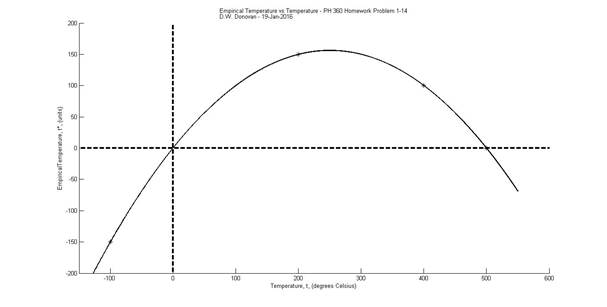
(a) Compute the emf when t = -100°C, 200°C, 400°C, and 500°C, and sketch a graph of versus t.

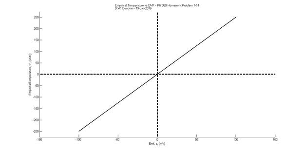
(b) Suppose the emf is taken as a thermometric property and that a temperature scale t* is defined by the linear equation:

Let t* = 0 at the ice point, and t* = 100 at the steam point. Find the numerical values of a and b and sketch a graph of versus t*.

(d) Is the t* scale a Celsius scale? Does it have any advantage or disadvantage compared with the IPTS scale?

Solution

(a) Compute the emf when t = -100°C, 200°C, 400°C, and 500°C, and sketch a graph of versus t.

, .

Using MATLAB, the desired values are found:

t (°C)	E (mV)
-100	-60
200	+60
400	+40
500	0

Graph of E vs t (note: Your graph should be a full page)

(b) Suppose the emf is taken as a thermometric property and that a temperature scale t* is defined by the linear equation:

Let t* = 0 at the ice point, and t* = 100 at the steam point. Find the numerical values of a and b and sketch a graph of versus t*.

First plug in for E, the relationship and we get:

Now we can plug in t* = 0 at the ice point (ie. t =0 °C), and t* = 100 at the steam point (ie. t = 100 °C).

At the ice point we get:

This reduces to

Which means b = 0.

Now plugging in for steam point:

So:

Plotting this in MATLAB (again work turned in should be a full page graph)

(c) Find the values of t* when t = -100°C, 200°C, 400°C, and 500°C, and sketch a graph of t* versus t over this range.

Plugging in the equation for E

Simplifying:

Using MATLAB, the desired values are found:

t (°C)	t*
-100	-150
200	150
400	100
500	0

Now we can plot this in MATALB

(d) Is the t* scale a Celsius scale? Does it have any advantage or disadvantage compared with the IPTS scale?

Since t* = 0 at t = 0°C and t* = 100 at t = 100°C, it can be considered a Celsius scale.

The Advantage compared to IPTS scale is the temperature can be calculated directly, rather than interpolated.

The Disadvantage is that a particular emf provides two temperatures and not just one.

MATLAB code for this problem follows:

%Solution to PH 360 Homework problem 1-14

%version 2016-01-19 D.W. Donovan

clear all;

a = 0.50;

b = -1e-3 ;

ta = [-100 200 400 500]';

Emfa =a*ta + b*ta.^2;

Ansa = [ta Emfa]

tap =[-150:0.001:550]';

Emfp = a*tap + b*tap.^2;

ac = 2.5;

Emfc =[-100:0.001:100]';

tstarc = ac*Emfc;

tstard = 1.25*ta-2.5e-3*ta.^2;

tstardp = 1.25*tap-2.5e-3*tap.^2;

ansd = [ta tstard]

anse = 1.25*(100)-2.5e-3*(100).^2

xx = [-150 600]';

yx = [0 0]';

xy = [0 0]';

yy = [-100 100]';

figure

hold on;

plot (ta, Emfa, 'k*', 'MarkerSize',8)

plot (tap,Emfp, 'k-', 'LineWidth',2)

plot (xx, xy, 'k--', 'LineWidth',3)

plot (xy, yy, 'k--', 'LineWidth',3)

axis ([-150 600 -100 100]);

xlabel('Temperature, t, (degrees Celsius)');

ylabel('Emf, \epsilon, (mV)');

tt1a=('Emf vs Temperature - PH 360 Homework Problem 1-14');

tt2='D.W. Donovan - ';

tta=[tt1a,'\newline',tt2,date];

title(tta)

figure

hold on;

plot (Emfc, tstarc,'k-','LineWidth',2)

plot (3*xx, 3*xy, 'k--', 'LineWidth',3)

plot (3*xy, 3*yy, 'k--', 'LineWidth',3)

axis ([-150 150 -275 275]);

ylabel('EmpiricalTemperature, t*, (units)');

xlabel('Emf, \epsilon, (mV)');

tt2a=('Empirical Temperature vs EMF - PH 360 Homework Problem 1-14');

tt2='D.W. Donovan - ';

ttc=[tt2a,'\newline',tt2,date];

title(ttc)

figure

hold on;

plot (ta, tstard, 'k*', 'MarkerSize',8)

plot (tap,tstardp, 'k-', 'LineWidth',2)

plot (2*xx, 2*xy, 'k--', 'LineWidth',3)

plot (2*xy, 2*yy, 'k--', 'LineWidth',3)

axis ([-150 600 -200 200]);

xlabel('Temperature, t, (degrees Celsius)');

ylabel('EmpiricalTemperature, t*, (units)');

tt3d=('Empirical Temperature vs Temperature - PH 360 Homework Problem 1-14');

tt2='D.W. Donovan - ';

ttd=[tt3d,'\newline',tt2,date];

title(ttd)

Ansa =

-100 -60

200 60

400 40

500 0

ansd =

-100 -150

200 150

400 100

500 0

anse =

100