|
|
|||||||||||||||
|
|
|||||||||||||||
|
4. Fitting non-polynomials #1 -
Trig functions |
|||||||||||||||
|
|
|||||||||||||||
|
For this problem you are to use the
data file lincrvtrigh.mat. This is in
the previously mentioned zip file found on my classes webpage. |
|||||||||||||||
|
|
|||||||||||||||
|
a) Find the parameters ( a3,
a2, a1, and a0) and the sum of squares (ss)
and the sum of squares per data point (ssdp) for the function:
|
|||||||||||||||
|
|
|||||||||||||||
|
|||||||||||||||
|
|
|||||||||||||||
|
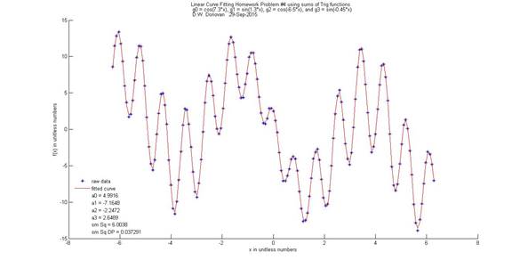
b) Produce a plot showing the raw data
and the fitted curve. You should
produce a legend which places the data from the above table onto the plot in
a place that obscures the data and the plot as little as possible. |
|||||||||||||||
|
|
|||||||||||||||
|
|
|||||||||||||||
|
|
|||||||||||||||
|
%Program
to Solve Problem 4 for Linear Curve Fitting Homework %version
2011-10-10 D.W. Donovan clear all; load('lincrvtrigh.mat','-ascii'); x=lincrvtrigh(:,1); fx=lincrvtrigh(:,2); g0=cos(7.3*x); g1=sin(1.3*x); g2=cos(-6.5*x); g3=sin(-0.45*x); al00=g0'*g0; al01=g0'*g1; al02=g0'*g2; al03=g0'*g3; al10=al01; al11=g1'*g1; al12=g1'*g2; al13=g1'*g3; al20=al02; al21=al12; al22=g2'*g2; al23=g2'*g3; al30=al03; al31=al13; al32=al23; al33=g3'*g3; b0=fx'*g0; b1=fx'*g1; b2=fx'*g2; b3=fx'*g3; alpha3=[al00
al01 al02 al03; al10 al11 al12 al13; al20 al21 al22 al23; al30 al31 al32 al33]; B3=[b0 b1 b2
b3]'; A3=alpha3\B3; p3=A3(1)*g0+A3(2)*g1+A3(3)*g2+A3(4)*g3; er3=p3-fx; ss3=er3'*er3; name='D.W.
Donovan'; tt31='Linear
Curve Fitting Homework Problem #4 using sums of Trig functions'; tt32='g0 =
cos(7.3*x), g1 = sin(1.3*x), g2 = cos(-6.5*x), and g3 = sin(-0.45*x)'; tt3=[tt31,' ',' \newline ',tt32,' \newline ',name,' ',date]; l3a0=['a0 = ',num2str(A3(1))]; l3a1=['a1 = ',num2str(A3(2))]; l3a2=['a2 = ',num2str(A3(3))]; l3a3=['a3 = ',num2str(A3(4))]; l3ss=['sm Sq = ',num2str(ss3)]; l3ssdp=['sm Sq DP = ',num2str(ss3/size(fx,1))]; figure hold on; title(tt3); xlabel('x in unitless numbers') ylabel('f(x) in unitless numbers') plot(x,fx,'b*') plot(x,p3,'r') plot(max(x),min(fx),'w.') plot(max(x),min(fx),'w.') plot(max(x),min(fx),'w.') plot(max(x),min(fx),'w.') plot(max(x),min(fx),'w.') plot(max(x),min(fx),'w.') legend('raw data','fitted curve',l3a0,l3a1,l3a2,l3a3,l3ss,l3ssdp,3); legend('boxoff') Sol={'a0 = ' A3(1); 'a1 = ' A3(2); 'a2 = ' A3(3); 'a3 = ' A3(4); 'sm Sq = ' ss3; 'sm Sq DP = '
(ss3/size(fx,1))}; Sol %{ Sol = 'a0 = ' [ 4.9916] 'a1 = ' [-7.1648] 'a2 = ' [-2.2472] 'a3 = ' [ 2.6489] 'sm Sq = ' [
6.0038] 'sm Sq DP = ' [
0.0373] %} |
|||||||||||||||
|
|||||||||||||||
|
|
|||||||||||||||
|
|