|
|
|||||||||||||||||||||||||||
|
|
|||||||||||||||||||||||||||
|
5. Non-Linear Two Lorentzian
Functions |
|||||||||||||||||||||||||||
|
|
|||||||||||||||||||||||||||
|
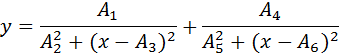
Use the file “nltwolor.mat”, it
contains data that should be fitted to a function of the form:
|
|||||||||||||||||||||||||||
|
|
|||||||||||||||||||||||||||
|
|||||||||||||||||||||||||||
|
|
|||||||||||||||||||||||||||
|
|
|||||||||||||||||||||||||||
|
|
|||||||||||||||||||||||||||
|
|
|||||||||||||||||||||||||||
|
|
|||||||||||||||||||||||||||
|
|
|||||||||||||||||||||||||||
|
|
|||||||||||||||||||||||||||
|
%Program
to solve non-linear Curve homework problem #5 %data
for a function F=a1/(a2^2+(x-a3)^2)+a4/(a5^2+(x-a6)^2 %version
2015-09-30 D.W. Donovan clear all; load('nltwolor.mat','-ascii'); x=nltwolor(:,1); fx=nltwolor(:,2); figure hold on; t1b='Non-Linear
Curve Fitting Homework Problem #5'; t2b='Raw Data to
be Fitted to F(x) = a1/(a2^2+(x-a3)^2)+a4/(a5^2+(x-a6)^2)'; name='D.W.
Donovan - '; tb=[t1b,'\newline',t2b,'\newline',name,date]; title(tb) xlabel('x in unitless numbers') ylabel('f(x) in unitless numbers') plot(x,fx) a00=[3000 8
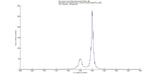
1200 4000 3.5 1350]; a=fminsearch(@nlh5pf,a00); a1=a(1); a2=a(2); a3=a(3); a4=a(4); a5=a(5); a6=a(6); ffx1=a1./(a2.^2+(x-a3).^2); ffx2=a4./(a5.^2+(x-a6).^2); ffx=ffx1+ffx2; ss=(fx-ffx)'*(fx-ffx); xc=[min(x):(max(x)-min(x))/100:max(x)]'; fxc1=a1./(a2.^2+(xc-a3).^2); fxc2=a4./(a5.^2+(xc-a6).^2); fxc=fxc1+fxc2; la00=['a00 = ',num2str(a00)]; la1=['a1 = ',num2str(a1)]; la2=['a2 = ',num2str(a2)]; la3=['a3 = ',num2str(a3)]; la4=['a4 = ',num2str(a4)]; la5=['a5 = ',num2str(a5)]; la6=['a6 = ',num2str(a6)]; lss=['sm Sq = ',num2str(ss)]; lssdp=['sm Sq DP = ',num2str(ss/size(fx,1))]; figure hold on; t1='Non-Linear
Curve Fitting Homework Problem #5'; t2='Data Fitted
to F(x) = a1/(a2^2+(x-a3)^2)+a4/(a5^2+(x-a6)^2)'; t=[t1,'\newline',t2,'\newline',name,date]; title(t) xlabel('x in unitless numbers') ylabel('f(x) in unitless numbers') plot(x,fx,'r*') plot(xc,fxc,'b') plot(min(xc),max(fxc),'w') plot(min(xc),max(fxc),'w') plot(min(xc),max(fxc),'w') plot(min(xc),max(fxc),'w') plot(min(xc),max(fxc),'w') plot(min(xc),max(fxc),'w') plot(min(xc),max(fxc),'w') plot(min(xc),max(fxc),'w') plot(min(xc),max(fxc),'w') legend('raw data','fitted curve',la00,la1,la2,la3,la4,la5,la6,lss,lssdp,2); legend('boxoff') Sol={'parameter' 'Start' 'End'; 'a1 = ' a00(1) a1; 'a2 = ' a00(2) a2; 'a3 = ' a00(3) a3; 'a4 = ' a00(4) a4; 'a5 = ' a00(5) a5; 'a6 = ' a00(6) a6; 'sm Sq = ' 'n/a' ss; 'sm Sq DP = ' 'n/a' (ss/size(fx,1))}; Sol %{ Sol = 'parameter' 'Start' 'End' 'a1 = ' [
3000] [2.9453e+03] 'a2 = ' [ 8]
[ 7.7802] 'a3 = ' [
1200] [1.2502e+03] 'a4 = ' [
4000] [3.9799e+03] 'a5 = ' [3.5000] [
3.8828] 'a6 = ' [
1350] [1.2999e+03] 'sm Sq = ' 'n/a'
[1.2754e+04] 'sm Sq DP = ' 'n/a' [ 25.4561] %} |
|||||||||||||||||||||||||||
|
%Function
m-file needed to solve nonlinear Curve fitting homework #3 %version
2007-10-08 D.W. Donovan function f = fun(a) load('nltwolor.mat','-ascii'); x=nltwolor(:,1); fx=nltwolor(:,2); a1=a(1); a2=a(2); a3=a(3); a4=a(4); a5=a(5); a6=a(6); g1=a1./(a2.^2+(x-a3).^2); g2=a4./(a5.^2+(x-a6).^2); g=g1+g2; f=(g-fx)'*(g-fx); |
|||||||||||||||||||||||||||
|
|||||||||||||||||||||||||||
|
|
|||||||||||||||||||||||||||
|
|